We live in a rapidly changing world with ever-increasing human impacts on natural systems. These impacts can look like increased harvesting pressures, encroachment on wild spaces, or human-driven changes to the climate, e.g., ocean acidification. As a result, natural populations are experiencing rapid change and decline/collapse ([1, 2]). In order to manage and conserve populations into the future, we must understand and even anticipate upcoming changes in population dynamics. This is a difficult task for many reasons, and explicitly considering a population's spatial distribution adds to this difficulty. Ecological data are expensive to gather, are often sparsely available over space and/or time, and naturally contain errors and/or missing data. Given these challenges, we seek to quantify dynamical changes in populations over time by quantifying changes in population distribution patterns over time, even when the data are sparsely available and/or contain only coarse-grain information like presence/absence data. The motivation for this work is the following: Given coarse-grain information on population distribution patterns, can just a few measurements in time be used to detect impending global extinction?
We use topological invariants called Betti numbers to quantify the population distribution patterns as they change over time. The data we use are cubical in nature (occurring on a grid/lattice) and spatially 2-dimensional, so we employ cubical homology and compute the first and second Betti numbers, \(\beta_0\) and \(\beta_1\) (for more information on computational homology, see [3]). For a given 2-dimensional cubical pattern, e.g., the set of cubes/patches where a species is present, \(\beta_0\) and \(\beta_1\) count the number of zero- and one-dimensional holes, respectively. More intuitively, \(\beta_0\) gives the number of "connected components" in the pattern (the number of distinct occupied regions), while \(\beta_1\) quantifies the number of unoccupied regions completely enclosed by occupied regions (i.e., holes). The first number, \(\beta_0\), naturally quantifies the level of fragmentation in a pattern and is thus particularly useful for ecological applications. As a proof of concept, we first show Betti numbers on spatial population model outputs as the modeled population experiences a global extinction event. In earlier work ([4, 5]), we found that topological information can provide a strong warning signal of impending global extinction.
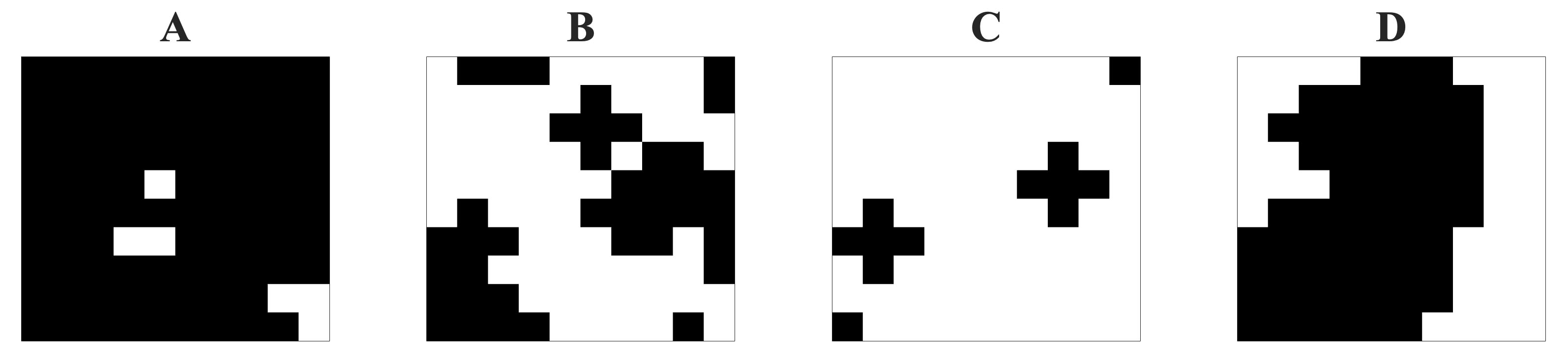
Figure 1. Example population distribution patterns on \(10 \times 10\) lattices. Black indicates that a patch is occupied (presence), white indicates that a patch is unoccupied (absence). We compute Betti numbers of the occupied set. A one-dimensional hole must be surrounded by occupied patches in order to count as a hole. Because patches are closed, occupied patches that are connected diagonally are part of the same connected component. In population A, there is one connected component and two holes (\(\beta_0 = 1\) and \(\beta_1 = 2\)). In population B there are five connected components and one hole (\(\beta_0 = 5\) and \(\beta_1 = 1\)). In population C there are 4 connected components and zero holes (\(\beta_0 = 4\) and \(\beta_1 = 0\)). In population D there is one connected component and zero holes (\(\beta_0 = 1\) and \(\beta_1 = 0\)).
Figure 1 displays some example population distribution patterns in the form of presence/absence data, where a white patch has zero population (absence) and a black patch has some nonzero population (presence). The Betti numbers for the sample images are provided in the caption. One may also threshold greyscale abundance data so that white indicates a patch with abundance at or below a given threshold and black indicates a patch with abundance above that threshold. However, in tracking global extinction events, presence/absence is a natural choice.
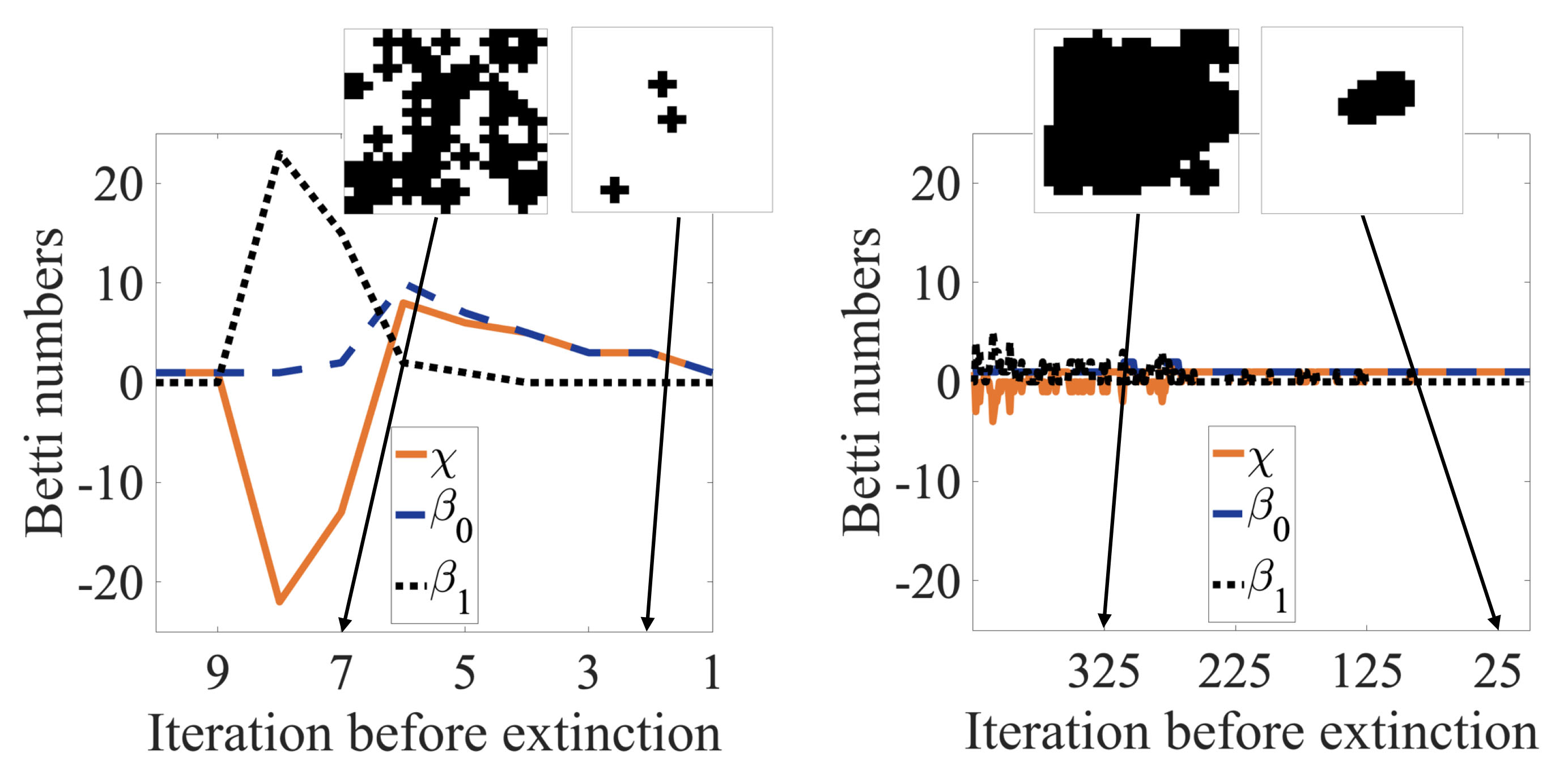
Figure 2. Example extinction events from a modeled population. The left image shows a fragmentation extinction event that occurs in 10 iterations/generations, and the right image shows a shrinking component extinction event that occurs in \(\approx400\) iterations (same initial conditions, different model parameters). Example population distribution patterns en route to extinction are displayed above the Betti number time series for each trial. On the left, the Euler characteristic curve displays a down-up-down pattern. On the right, the Betti number time series shows some "flickering" in \(\beta_1\) as one-dimensional holes are formed and destroyed, but the Betti number time series remains largely steady, especially for the last 100 iterations.
Figure 2 shows two example Betti number time series of modeled population extinction events. We use a discrete time coupled patch population model to produce the population distribution time series ([5]). These populations were modeled on \(21 \times 21\) lattices representing patches in space, with each iteration of the model representing one generation of the population. In addition to calculating \(\beta_0\) and \(\beta_1\) we also calculate the Euler characteristic, \(\chi = \beta_0 - \beta_1\). The first panel shows fragmentation, a rapid extinction event for this model in which the population uniformly fragments across the lattice. The Betti numbers and Euler characteristic display a dramatic and characteristic shape as the population heads toward global extinction. The second panel of figure 2 shows a relatively slow extinction event for this model that we label shrinking component. In this second scenario, the spatial extent of the population (maximum Euclidean distance between occupied patches) slowly shrinks over time. Here, a measure of spatial extent or something similar is needed to track the global extinction event, since the Betti number and Euler characteristic time series remain relatively constant (this is due to the fact that there is a single connected component that is shrinking over time, and the Betti numbers don't measure information about the spatial scale of the connected component). Extinction events that look like a mix of fragmentation and shrinking component were also observed, yielding a continuum of extinction routes between these two extremes.
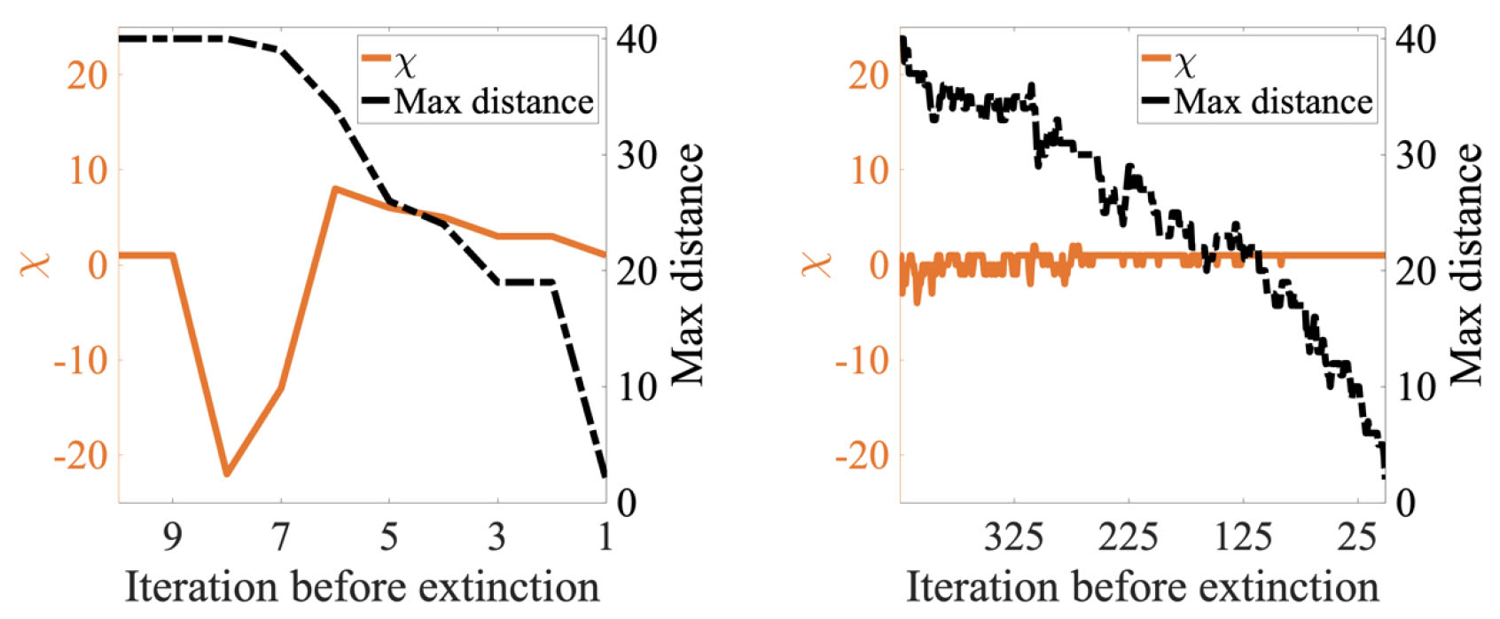
Figure 3. For the two example extinction events in figure 2, we plot the Euler characteristic against the maximum Euclidean distance between occupied patches en route to extinction. We observe that for the fragmentation route to extinction (left plot), the max distance remains steady for several iterations while the Euler characteristic begins a dramatic decline. Thus, for this rapid route to extinction, the topological early warning signal provides an earlier indication of impending change than a more straight-forward metric. For the shrinking component route to extinction (right plot), the Euler characteristic jitters at the beginning of the time series but is largely flat, while the max distance slowly decreases over time, providing a warning that something is occurring to the population.
Figure 3 shows the measure of spatial extent for both extinction examples along with the Euler characteristic time series for comparison.
We observe that in the rapid fragmentation extinction event, the Betti numbers/Euler characteristic provide an earlier warning signal that change is occurring than the spatial extent. In the first few iterations of the model run, the Euler characteristic begins its dramatic dive while the spatial extent remains relatively steady. Thus we argue that topological quantification of the population distribution patterns can provide useful information in early detection of impending change in a population. These topological measures can also give a clear signal of impending change based on very coarse-grain data (e.g., presence/absence) that are more likely to be available to ecologists.
While both extinction types are well-studied in the ecological literature (e.g., [6]) we now focus on the most rapid extinction type - extinction via fragmentation - and ask the question of how quickly we can determine that a population will end up going extinct. Towards this goal, summer research intern Paige Bilich (Bates College class of 2026) studied patterns generated by the voter model, which exhibits fragmentation but not shrinking component extinction.
1. A first example: the voter model
As a first exploration of using Betti numbers in early detection of global extinction via fragmentation, we turn to patterns generated by the voter model. As the name suggests, the voter model is often used to simulate the spread of opinions and voting trends. Patches are either black or white, which can represent presence/absence, two different political opinions, etc. A patch on the lattice becomes black or white in the next model iteration depending on the colors of the four nearest neighbors plus a bias in the model. The bias can be set to 0.5 for no bias towards black or white, or set to a different probability to prefer black or white. We utilized the biased voter model ([7, 8]) to allow for white/absent patches to eventually dominate, signaling an "extinction" of black/occupied patches.
The chances of the \(i,j\)th patch becoming black or white is dictated by:
| |
\( \begin{split}
P(s_{i,j} \to 0) = \frac{bn^{(0)}_{i,j}}{bn^{(0)}_{i,j} +(1-b)n^{(1)}_{i,j}} \\
P(s_{i,j} \to 1) = \frac{(1-b)n^{(1)}_{i,j}}{bn^{(0)}_{i,j} +(1-b)n^{(1)}_{i,j}}
\end{split} \) |
(1) |
respectively, where \(s_{i,j}=0\) if the patch is white, \(s_{i,j}=1\) if the patch is black, \(n^{(0)}_{i,j}\) is the number of surrounding four patches that are white, \(n^{(1)}_{i,j}\) is the number of surrounding four patches that are black, and \(0\leq b \leq 1\) is the bias ([7, 8]).
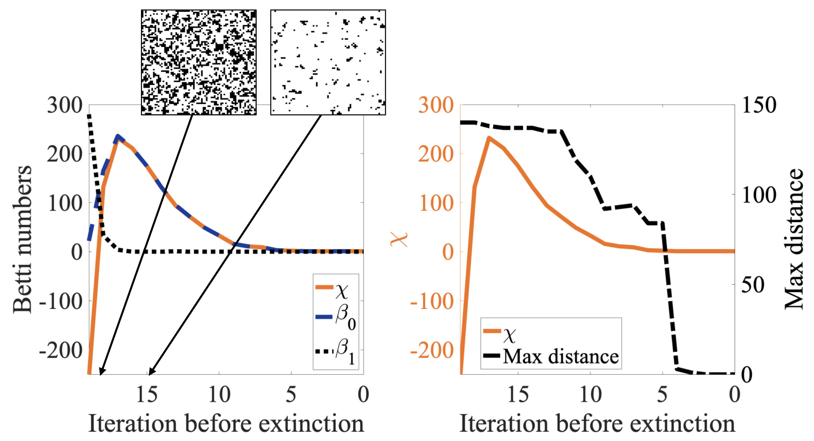
Figure 4. An example Betti number time series of an "extinction event" (domination of one color) in the biased voter model (left plot). We observe that the Betti numbers are larger than in figure 2 because this model was on a larger lattice than the coupled patch model (\(71 \times 71\) versus \(21 \times 21\)). In this model run, we begin with a random initial condition in which roughly 50% of patches are black and 50% are white, and the bias in favor of white patches is set to 0.7. The white patches quickly begin to dominate and we observe a fragmentation-like extinction event, with a dramatic decrease in \(\beta_1\) followed by an increase then decrease in \(\beta_0\). In the right plot we show the Euler characteristic, \(\chi\), with the maximum Euclidean distance between black patches, as in figure 3. Once again we observe that the spatial extent of the black patches doesn't provide as early of a warning signal as \(\chi\).
Figure 4 shows an example Betti number and Euler characteristic time series for the voter model in the left plot, and Euler characteristic and spatial extent/max distance in the right plot. This example shows an "extinction event" in the voter model, in which the white patches dominate and the black patches go extinct. Starting with a mixed black/white initial condition with negative Euler characteristic, we observe similar patterns in the Betti numbers and Euler characteristic following initial hole formation for the coupled-patch model, e.g., around iterate 8 before extinction in figure 2.
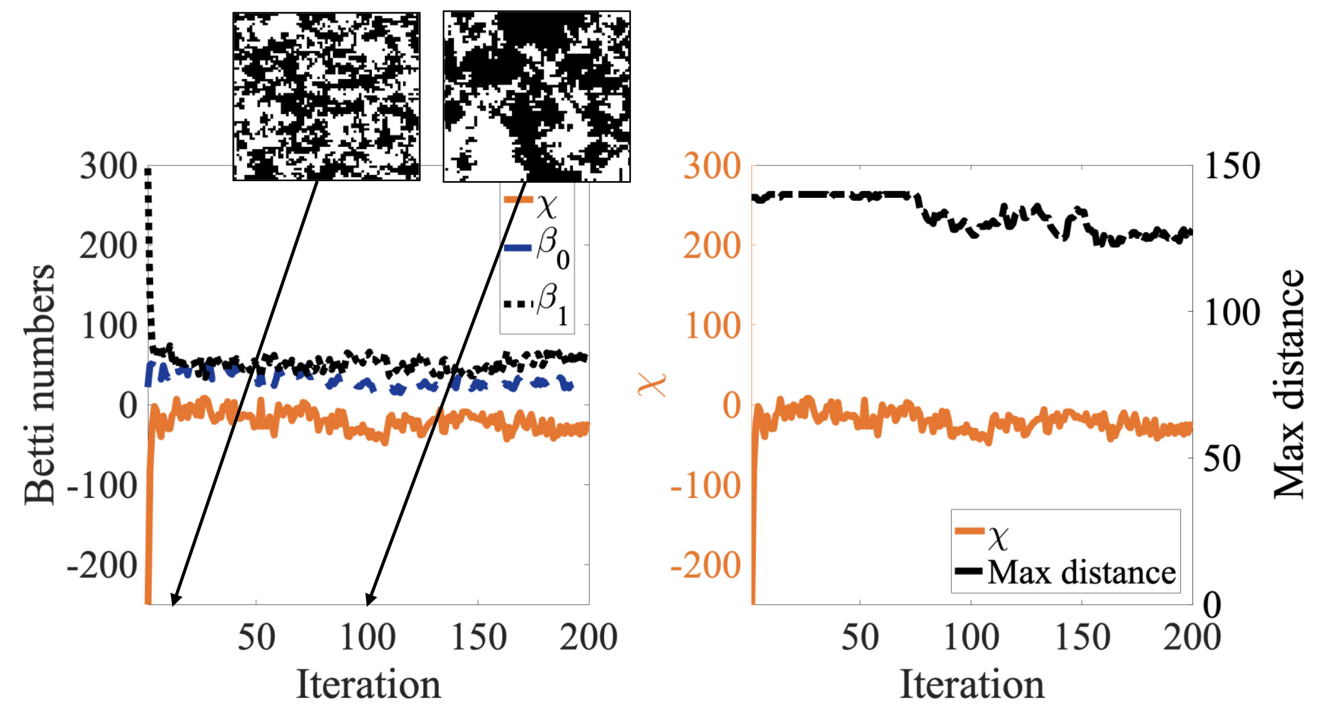
Figure 5. An example Betti number time series of persistence (non-extinction) in the biased voter model, i.e., both black and white patches persist (left plot). We observe that the Betti numbers are larger than in figure 2 because this model was run on a larger lattice than the coupled patch model (\(71 \times 71\) versus \(21 \times 21\)). In this model run, we begin with a random initial condition in which roughly 50% of patches are black and 50% are white, and the bias is set to 0.5 (no bias). In the right plot we show \(\chi\) with the maximum Euclidean distance between black patches, as in figure 3. The length of the time series is 1001 iterations, but we show only the first 200 iterations to better illustrate the "jittering" in \(\beta_0\), \(\beta_1\), and the spatial extent over time (the rest of the time series is qualitatively similar).
Figure 5 shows an example of persistence of both colors in the voter model with no global extinction. Here, we observe that the Betti numbers and max distance largely "jitter" and remain at similar values. In the beginning there is a decrease in \(\beta_1\) as the original random condition looks like static, and as the model iterates forward in the first few iterations the black and white patches become more clumped in appearance.
For Paige's project, she computed Betti number time series on 745 model runs in which there were global extinction events and 645 model runs in which the population persisted (i.e. both colors remained) after 1000 model iterations (1390 total trials). The average length of a time series that went extinct was \(\approx\) 43 iterations. Paige tested the ability of machine learning algorithms to properly categorize time series as going extinct versus persisting, using Betti numbers from 3 early iterations of the model runs. Some time series only persisted for \(\approx\) 10 iterations before extinction, and so we were limited in the information we could feed the machine learning algorithms. As a preliminary experiment, we tested the predictive power of the Betti numbers from iterations \((1,2,3)\) and \((2,3,4)\), where the zeroth iteration is the initial condition. Using early and few iterations also makes sense ecologically, as ecological measurements are costly and difficult to obtain.
XGBoost and K Nearest Neighbors algorithms were selected due to their ability to make predictions with smaller training sets ([9, 10]). XGBoost is a supervised machine learning algorithm and uses decision trees and combines their results to create a higher performing model. K-Nearest Neighbors is also a supervised machine learning algorithm used for classification. It uses Euclidean distance to calculate the distance between data points and classifies new data points based on the closest k neighbors. 80% of the 1390 model runs were randomly selected as the training data and the remaining 20% of model runs were used for prediction. The algorithms were only fed information from the chosen set of iterations ((1,2,3) or (2,3,4)) for training. We observe from the figures of extinction versus persistence (figures 4 and 5) that the Betti numbers are quite different and so we would expect the machine learning to perform well, and it does (classification accuracy of \(\approx\) 95% and above). Given that the average time to extinction was 43 iterations, using information from just the first few iterations for this highly accurate classification yields a promising early warning signal for extinction.
While a few early coarse-grain measurements worked well to predict eventual extinction/persistence in the voter model, more study is required to bridge the gap between these model simulations and real world patterns. Indeed, returning to the coupled-patch model with its topologically distinct routes to extinction (fragmentation versus shrinking component, as well as mixtures of the two) will already present an interesting challenge to these methods. Ultimately, finding a way to translate sparse and coarse spatial measurements into useful predictions of long term population persistence or extinction will greatly aide forecasting efforts in real world ecological systems.
References
[1] J. F. McLaughlin, J. J. Hellmann, et al., Climate change hastens population extinctions, Proceedings of the National Academy of Sciences, 99(9), pp. 6070-6074, 2002.
[2] S. H. M. Butchart, M. Walpole, et al., Global Biodiversity: Indicators of Recent Declines, Science, 328(5982), pp. 1164-1168, 2010.
[3] T. Kaczynski, K. Mischaikow, and M. Mrozek, Computational Homology, Springer, 2004.
[4] L. S. Storch and S. L. Day, Towards the prediction of critical transitions in spatially extended populations with cubical homology, Contemporary Mathematics, 736, pp. 31-48, 2019.
[5] L. S. Storch and S. L. Day, Topological early warning signals: Quantifying varying routes to extinction in a spatially distributed population model, Journal of Theoretical Biology, 554, 111274, 2022.
[6] R. Channell and M. V. Lomolimo, Trajectories to extinction: Spatial dyanmics of the contraction of geographic ranges, Journal of Biogeography, 27(1), pp. 169-179, 2000.
[7] A. Czaplicka, C. Charalambous, et al., Biased-voter model: How persuasive a small group can be?, Chaos, Solitions, & Fractals, 161, 112363, 2022.
[8] P. Mullick and P. Sen, Social influence and consensus building: Introducing a q-voter model with weighted influence, PLoS One, 20(1), e0316889, 2025.
[9] M. Zou, Miao, W.-G. Jiang, Q.-H. Qin, Y.-C. Liu, and M.-L. Li, Optimized XGBoost Model with Small Dataset for Predicting Relative Density of Ti-6Al-4V Parts Manufactured by Selective Laser Melting, Materials, 15(15), 5298, 2022.
[10] J. Lin, Investigation Related to Performance of KNN, Logistic Regression and XGBoost on Diabetes Prediction, Proceedings of the 2023 International Conference on Image, Algorithms and Artificial Intelligence (ICIAAI 2023), pp. 670-676, 2023.