1. Introduction
NumbaCS (Numba Coherent Structures) is a fast, open-source Python package for computing Lagrangian and objective Eulerian coherent structures in time-dependent flows. It combines high computational performance (achieved by leveraging Numba -- a just-in-time compiler for Python) with an accessible Python interface to offer a powerful and user-friendly platform for analyzing transport in geophysical, environmental, and engineered systems. This combination of performance and accessibility makes it an ideal tool for a wide range of users, from seasoned researchers to those new to the field.
Lagrangian coherent structures (LCS) [Haller and Poje(1998), Shadden et al.(2005), Haller(2011), Farazmand and Haller(2012), Haller et al.(2016)], and more recently objective Eulerian coherent structures (OCES) [Serra and Haller(2016), Haller et al.(2016), Nolan et al.(2020)] -- their instantaneous counterparts, have emerged as key tools for understanding material transport in unsteady flows. By making use of linearizations around particle trajectories for the entire domain of interest, one can derive organizing structures that govern material transport in these complex flows. For more details on these methods, refer to the cited works or the Theory and Implementation section in the documentation for a brief overview.
While many great packages for computing coherent structures exist (see Similar software), we set out to create a modern package that implements a variety of methods and combines the speed of a compiled language with the ease-of-use of an interpreted language. By building NumbaCS on top of three key packages (Numba, numbasloda, and interpolation), we are able to achieve speeds approaching those of a compiled language while providing the user with a straightforward Python interface (see Key dependencies for more information on how this is achieved). Furthermore, since the package is written in pure Python, it offers a simple environment for community contributions and long-term maintenance.
2. Features & Functionality
Below we highlight some important features that make NumbaCS a robust package and then list the methods currently implemented.
Features
- Thorough documentation available online: numbacs.readthedocs.io.
- Many examples demonstrating functionality: Examples Gallery.
- Intuitive API: A function-based approach and reliance on standard NumPy arrays ensure a low barrier for entry.
- Hosted on public repositories (GitHub, PyPI, and conda-forge) allowing easy installation.
- Continuous integration to ensure the latest release is automatically tested across major platforms (Linux, MacOS, Windows) for stability and reliability.
- Designed around a modular workflow, allowing computationally expensive objects (e.g., flow maps) to be computed once and reused across multiple methods (e.g., FTLE, LAVD).
- High performance via just-in-time compilation.
- Core computations are automatically parallelized without the need for user configuration.
- Open source under the MPL 2.0 license to encourage collaboration while allowing easy integration with other software.
Functionality
NumbaCS implements the following methods for both analytical and numerical flows:
NumbaCS is actively being developed; see the Roadmap for planned methods and features.
3. Installation
NumbaCS can easily be installed
with conda: ```conda install -c conda-forge numbacs ```
or pip: ```pip install numbacs ```
We generally recommend users install with conda, as one of the dependencies occasionally has issues with pip (though this seems to primarily affect Windows builds).
4. Getting started and Examples
As mentioned, there is a large collection of examples in the Examples Gallery and we encourage users to start there to get accustom to the package. For a more detailed introduction, a user may refer to the User Guide, which provides a comprehensive guide to the workflow. In addition, there is an API reference with links to source code. Below, we link to several examples that highlight the power and utility of NumbaCS, along with accompanying figures where relevant.
4.1. FTLE ridges & Hyperbolic LCS
In the Double gyre FTLE ridges and Double gyre hyperbolic LCS examples, we show two ways to compute hyperbolic LCS in NumbaCS, namely by computing FTLE ridges (Figure 1, top) and variational hyperbolic LCS (Figure 1, bottom). We generally recommend using the FTLE ridge methods, as they are extremely fast and simpler for the user. That being said, for those who wish to use the variational hyperbolic LCS method, the implementation provided by NumbaCS is also quite fast.
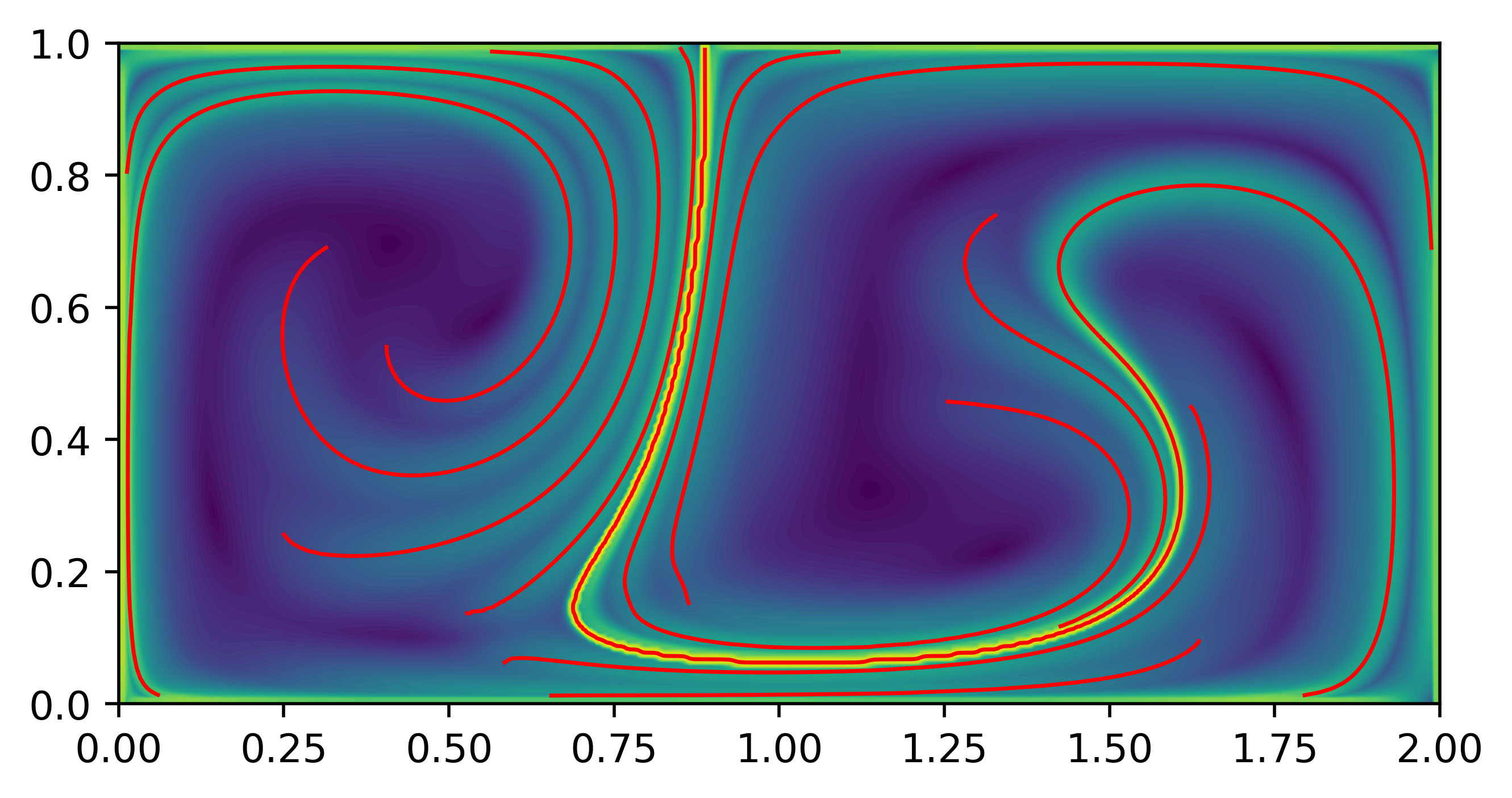
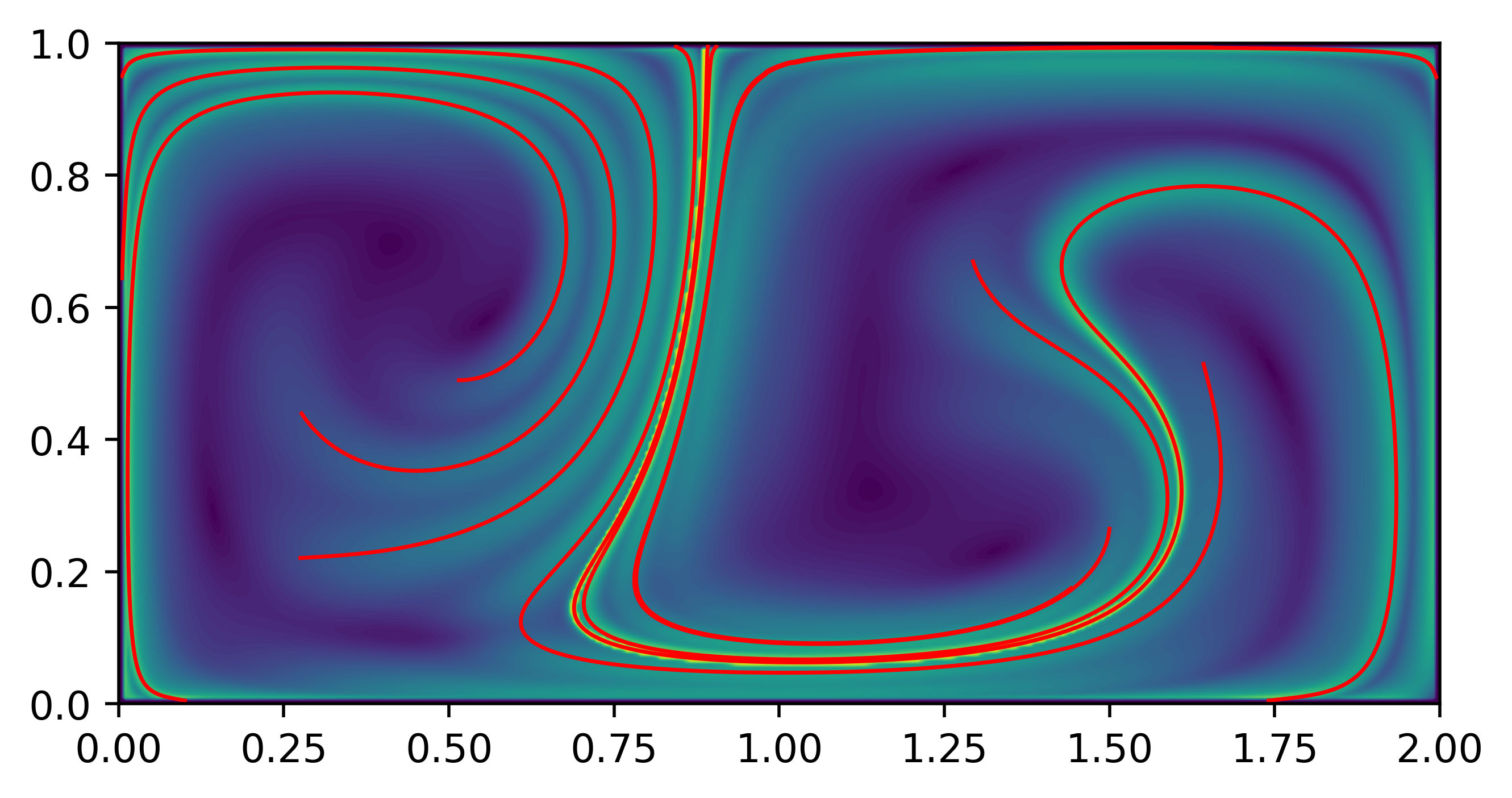
Figure 1. Top: DG backward FTLE ridges. Bottom: DG hyperbolic LCS. Both computed for integration time of \(T=-10\).
4.2. FTLE on the Sphere and masked support
In the MERRA-2 Globe FTLE and Copernicus Globe FTLE examples, we demonstrate how to compute FTLE on the sphere. The former uses reanalysis data provided by the NASA MERRA-2 product [Gelaro et al.(2017), GMAO(2015)] (more details can be found in the following paper [Jarvis et al.(2024)]), and the latter uses the Copernicus Global Ocean Ensemble Physics Reanalysis product [CMEMS(2024)], showcasing masked particle integration and FTLE support. In the left panel of Figure 2 we show backward FTLE computed using the MERRA-2 data, and in the right panel show forward FTLE computed using the Copernicus data.
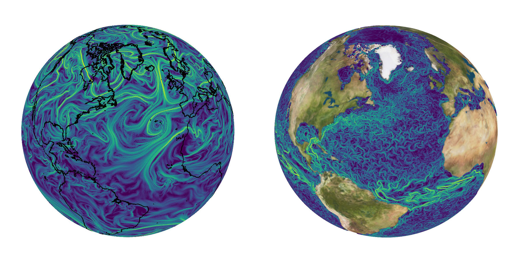
Figure 2. Left: Backward-time FTLE for integration time of -72 hours using MERRA-2 velocity data. Right: Forward-time masked FTLE for integration time of 60 days using Copernicus velocity data. Both on June 16, 2020.
4.3. LAVD & Elliptic LCS
In the Bickley jet Elliptic LCS example, we demonstrate how to compute the LAVD field and LAVD-based elliptic LCS. In Figure 3, the top panel shows the LAVD-based elliptic LCS overlaid on the LAVD field computed for the Bickley jet with an integration time of 40 days. The middle panel shows a specific elliptic LCS with some particles inside it and some nearby, and the bottom panel shows the advected images of these particles after 40 days. A video is provided in the linked example.
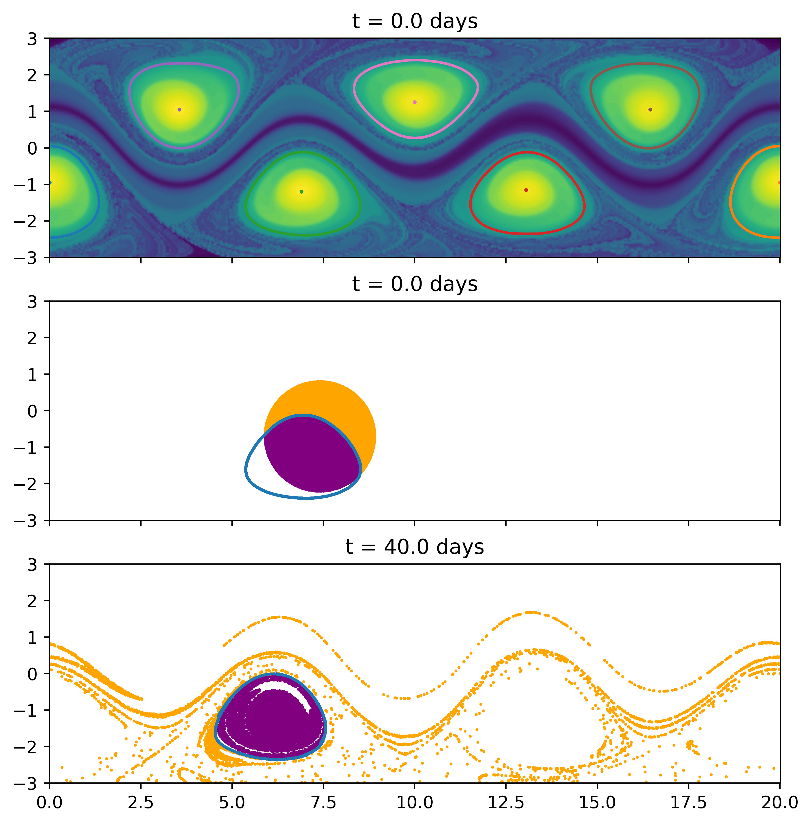
Figure 3. Top: LAVD-based elliptic LCS overlaid on LAVD field (integration time \(T = 40\) days). Middle: Initial positions of particles both in (purple) and around (orange) an ellptic LCS. Bottom: Final positions (after 40 days) of those same particles.
In the Quasi-geostrophic Elliptic LCS example, we show the same computation for the quasi-geostrophic equations. We thank the authors of Mou et al. [Mou et al.(2021)] for providing us with this dataset and graciously allowing a portion of it to be included with the package. In Figure 4, the left panel shows the LAVD-based elliptic LCS overlaid on the LAVD field computed for the QGE with an integration time of 0.3. The middle panel shows the identified elliptic LCS with some particles inside it and some nearby, and the bottom panel shows the advected images of these particles after 0.3 units of time. A video is provided in the linked example.
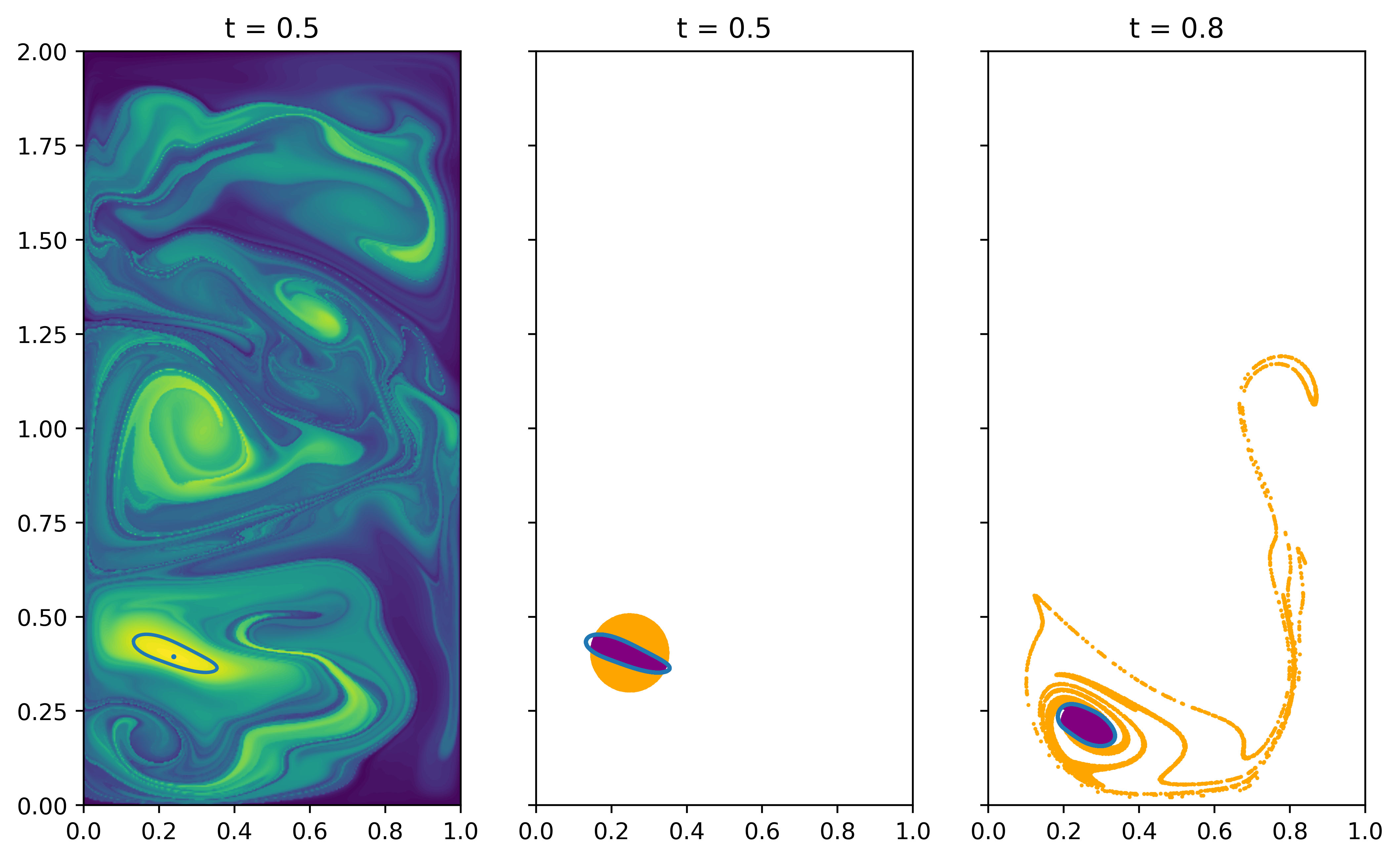
Figure 4. Top: LAVD-based elliptic LCS overlaid on LAVD field (integration time \(T = 0.3\)). Middle: Initial positions of particles both in (purple) and around (orange) an ellptic LCS. Bottom: Final positions (after 0.3 units of time) of those same particles.
4.4. iLE and Hyperbolic OECS
In the Quasi-geostrophic hyperbolic OECS example, we demonstrate how to compute the ilE field and hyperbolic OECS. In the left panel of Figure 5, we show hyperbolic OECS saddle cores overlaid on the iLE field. In the remaining panels of Figure 5, we show the initial and advected images of particles centered at the three strongest objective saddle points for a short integration time.
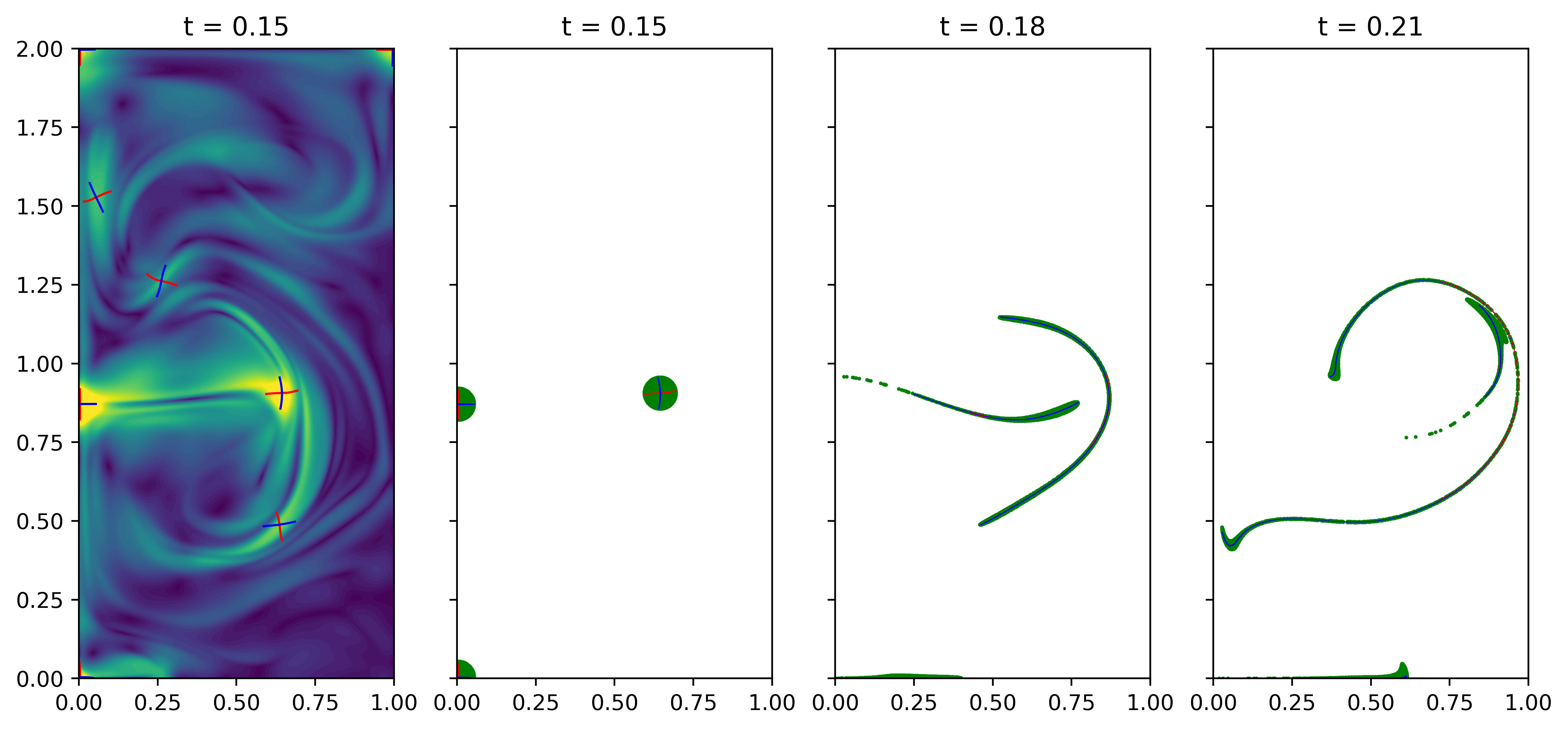
Figure 5. Left: Hyperbolic OECS overlaid on iLE field. Middle-left: Initial positions three strongest hyperbolic OECS (red and blue) and circle of particles surrounding them (green). Middle-right: Image those particles after 0.03 units of time. Right: Image of those particles after 0.06 units of time.
4.5. Time series and Flow map composition
Since NumbaCS relies heavily on Numba for speed, many of the provided functions are compiled just-in-time. As a result, the first function call is generally noticeably slower than subsequent calls. Due to this, the power of NumbaCS is fully realized when computing diagnostics or feature extraction for a time series. In addition, NumbaCS provides an option to use a highly underutilized method to accelerate particle integration introduced by Brunton and Rowley [Brunton and Rowley(2010)], which we refer to as the flow map composition method (see the Flow map composition section in the documentation or refer to the cited paper for more details). In the Double gyre time series and Quasi-geostrophic time series examples, we demonstrate how to apply this method and highlight the expected speedups for flows defined by analytical equations and numerical velocity data, respectively. These examples also give users a rough estimate of the runtimes they can expect when using the standard methods.
5. Acknowledgments and Citation
This work was partially supported by the National Science Foundation (NSF) under grant number 1821145 and the National Aeronautics and Space Administration (NASA) under grant number 80NSSC20K1532 issued through the Interdisciplinary Research in Earth Science (IDS) and Biological Diversity & Ecological Conservation programs.
We also thank the reviewers and editors at the Journal of Open Source Software (JOSS) for their feedback and suggestions during the review process. The JOSS article provides a high-level overview of the package and its performance. If you use NumbaCS in your research, we kindly ask that you cite this paper [Jarvis and Ross(2025)].
References
[Brunton and Rowley(2010)] S. L. Brunton and C. W. Rowley, Fast computation of finite-time Lyapunov exponent fields for unsteady flows, Chaos: An Interdisciplinary Journal of Nonlinear Science, 20(1): 017503, 01 2010, ISSN 1054-1500, DOI: 10.1063/1.3270044.
[CMEMS(2024)] E.U. Copernicus Marine Service Information (CMEMS)}, Global Ocean Ensemble Physics Reanalysis, Marine Data Store (MDS), DOI: 10.48670/moi-00024.
[Farazmand and Haller(2012)] M. Farazmand and G. Haller, Computing Lagrangian coherent structures from their variational theory, Chaos: An Interdisciplinary Journal of Nonlinear Science, 22(1): 013128, 03 2012, ISSN 1054-1500, DOI: 10.1063/1.3690153.
[Gelaro et al.(2017)] R. Gelaro, W. McCarty, M. J. Suarez, R. Todling, A. Molod, L. Takacs, C. A. Randles, A. Darmenov, M. G. Bosilovich, R. Reichle, K. Wargan, L. Coy, R. Cullather, C. Draper, S. Akella, V. Buchard, A. Conaty, A. M. da Silva, W. Gu, G.-K. Kim, R. Koster, R. Lucchesi, D. Merkova, J. E. Nielsen, G. Partyka, S. Pawson, W. Putman, M. Rienecker, S. D. Schubert, M. Sienkiewicz, and B. Zhao, The Modern-Era Retrospective Analysis for Research and Applications, Version 2 (MERRA-2), Journal of Climate, American Meteorological Society, Boston MA, USA, 30(14): 5419-5454, 2017, DOI: 10.1175/JCLI-D-16-0758.1.
[GMAO(2015)] GMAO, Global Modeling and Assimilation Office, MERRA-2 inst3_3d_asm_Np: 3d, 3-Hourly, Instantaneous, Pressure-Level, Assimilation, Assimilated Meteorological Fields V5.12.4, Greenbelt, MD, USA, Goddard Earth Sciences Data and Information Services Center (GES DISC), 2015, DOI: 10.5067/QBZ6MG944HW0.
[Haller(2011)] G. Haller, A variational theory of hyperbolic Lagrangian Coherent Structures, Physica D: Nonlinear Phenomena, 240(7): 574-598, 2011, ISSN 0167-2789, DOI: 10.1016/j.physd.2010.11.010.
[Haller and Poje(1998)] G. Haller and A. Poje, Finite time transport in aperiodic flows, Physica D: Nonlinear Phenomena, 119(3): 352--380, 1998, ISSN 0167-2789, DOI: 10.1016/S0167-2789(98)00091-8.
[Haller et al.(2016)] G. Haller, A. Hadjighasem, M. Farazmand, and F. Huhn, Defining coherent vortices objectively from the vorticity, Journal of Fluid Mechanics, 795: 136–173, 2016, DOI: 10.1017/jfm.2016.151.
[Jarvis and Ross(2025)] A. Jarvis and S. D. Ross, NumbaCS: A fast Python package for coherent structure analysis, Journal of Open Source Software, 10(113): 7948, 2025, DOI: 10.21105/joss.07948.
[Jarvis et al.(2024)] A. Jarvis, A. Hossein Mardi, H. Foroutan, and S. D. Ross, Atmospheric transport structures shaping the "Godzilla" dust plume, Atmospheric Environment, 333: 120638, 2024, DOI: 10.1016/j.atmosenv.2024.120638.
[Lekien and Ross(2010)] F. Lekien and S. D. Ross, The computation of finite-time Lyapunov exponents on unstructured meshes and for non-Euclidean manifolds, Chaos: An Interdisciplinary Journal of Nonlinear Science, 20(1): 017505, 2010, DOI: 10.1063/1.3278516.
[Mou et al.(2021)] C. Mou, Z. Wang, D. R. Wells, X. Xie, and T. Iliescu, Reduced Order Models for the Quasi-Geostrophic Equations: A Brief Survey, Fluids, 6(1), 2021, ISSN 2311-5521, DOI: 10.3390/fluids6010016, URL: https://www.mdpi.com/2311-5521/6/1/16.
[Nolan et al.(2020)] P. Nolan, M. Serra, and S. D. Ross, Finite-time Lyapunov exponents in the instantaneous limit and material transport, Nonlinear Dyn, 100: 3825-3852, 2020, DOI: 10.1007/s11071-020-05713-4.
[Schindler et al.(2012)] B. Schindler, R. Peikert, R. Fuchs, and H. Theisel, Ridge Concepts for the Visualization of {L}agrangian Coherent Structures, Springer Berlin Heidelberg, Berlin, Heidelberg, 2012, pages 221-235, ISBN 978-3-642-23175-9, DOI: 10.1007/978-3-642-23175-9_15.
[Serra and Haller(2016)] M. Serra and G. Haller, Objective Eulerian coherent structures, Chaos: An Interdisciplinary Journal of Nonlinear Science, 26(5): 053110, 05 2016, ISSN 1054-1500, DOI: 10.1063/1.4951720.
[Shadden et al.(2005)] S. C. Shadden, F. Lekien, and J. E. Marsden, Definition and properties of Lagrangian coherent structures from finite-time Lyapunov exponents in two-dimensional aperiodic flows, Physica D: Nonlinear Phenomena, 212(3): 271-304, 2005, ISSN 0167-2789, DOI: 10.1016/j.physd.2005.10.007.
[Steger(1998)] C. Steger, An unbiased detector of curvilinear structures, IEEE Transactions on Pattern Analysis and Machine Intelligence, 20(2): 113-125, 1998, DOI: 10.1109/34.659930.